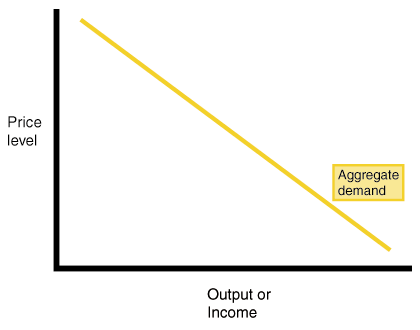
Aggregate Demand
- Shows the amount of Real GDP that the private, public, and foreign sector collectively desire to purchase at each possible price level.
- Relationship between the price level and level of GDPr is inverse
3 Reasons AD is downward sloping
- Real-Balances Effect
- Interest-Rate Effect
- Foreign Purchases Effect
Shifts in AD
- Change in C, Ig, G, or Xn
- Multiplier effect that produces a greater change than the original change in the 4 components
- Increase in AD, shift right
- Decrease in AD, shift left
Net Exports
- Exchange Rates (International value of U.S. dollar)
- Strong dollar = More imports and Less Exports = (AD shift left)
- Weak dollar = fewer imports and more exports = (AD shift right)
Relative Income
- Strong Foreign Economies = More Exports = AD shift right
- Weak Foreign Economies = Less Exports = AD shift left
Aggregate Supply
- The level of Real GDP that firms will produce at each price level

Long-Run v. Short-Run
- Long-Run
- Period of time where input prices are flexible and adjust to changes in the price-level
- In the long-run, the level of Real GDP is independent from price level
- Short-Run
- Period of time where input prices are sticky and do not adjust to changes in the price-level
- Real GDP is directly related to the price level
Long-Run Aggregate Supply (LRAS)
- marks the level of FE in the economy (same as the PPC)
- is always vertical at full employment
Changes in Short-Run Aggregate Supply (SRAS)
- increase in SRAS, shift to the right
- decrease, shift to the left
- the key to understanding shifts is per unit cost of production
- per-unit production cost = total input cost / total output
Determinants of SRAS
- Input prices = land, labor, machinery, ETC.
- Productivity = technology
Ranges of Aggregate Supply (AS)

Keynesian Range
- Horizontal
- Followers believe in a horizontal AS curve because when the economy is below FE, AD shifts out
- Increase in GDPr, UE drops, price level is constant
- Demand creates its own supply
Intermediate Range
- AS is between the Classical and Keynesian Range
- AS shifts outward, price level and GDPr increases
Classical Range
- Vertical
- In the long run, AS curve is vertical because the only effects of an increase in AD is when we are already at FE
- Increase in price level
- Supply creates its own demand (Say's Law)
Recessionary Gap - when equilibrium occurs below FE output

Inflationary Gap - when equilibrium occurs beyond FE output

Investment

- Money spent or expenditures on:
- New plants (factories)
- Capital equipment (machinery)
- Technology (hardware and software)
- New homes
- Inventories (goods sold by producers)
- Expected rates of return
- How does business make investment decisions?
- Cost/benefit analysis
- How does business determine the benefits?
- expected rate of return
- How does business count the cost?
- interest costs
- How does business determine the amount of investment they undertake?
- Compare expected rate of return to interest cost
- expected return > interest cost = invest
- expected return < interest cost = don't invest
- Real (r %) v. Nominal (i %)
- Nominal is the observable rate of interest
- Real subtracts out inflation and is only known ex post facto
- Compute r%
- = nominal - inflation
- Real interest rate (r%) determines the cost of investment decision
- Investment Demand Curve (ID)
- Downward sloping
- Why?
- when interest rate are high, fewer investments are profitable
- when ir are low, investments are profitable
- Shifts in ID
- Cost of production
- Business taxes
- Technology changes
- Stock of capital
- Expectations
- Consumption and Savings
- Disposable income (DI)
- income after taxes
- net imcome
- Consumption
- Household spending
- Ability to consume is constrained by: amount of DI and propensity to save
- DI = 0
- Dissaving
- Savings
- Household not spending
- Ability to save is constrained by: amount of DI and propensity to consume
- APS = average propensity to save
- APC = average propensity to consume
- APC + APS = 1
- APC > 1 dissaving
- MPC = marginal propensity to consume
- = change in consumption / change in DI
- MPS = marginal propensity to save
- = change in savings / change in DI
- MPS + MPC = 1
Determinants of C & S

- Wealth
- Expectations
- Household Debt
- Taxes
Spending Multiplier Effect
- an initial change in spending (C, Ig, G, Xn) causes a larger change in AD
- Multiplier - change in AD / change in spending
- 1 / MPS
- positive when increase in spending
- negative when decrease
Tax Multiplier
- when government taxes, the multiplier works in reverse
- money is leaving circular
- Multiplier (negative) = - MPC / MPS
Fiscal Policy
- Expansionary and Contractionary policy
- Deficits and surplus
- Built in stability
Changes in expenditures or tax revenues of the federal government
2 tools of fiscal policy
- Taxes - government can increase or decrease taxes
- Spending - government can increase/decrease spending
Fiscal policy is enacted to promote our nation's economic goods = FE, price stability, economic growth

Deficits, Surpluses, Debt
- Balanced Budget
- Revenues = Expenditures
- Budget deficit
- Revenues < expenditures
- Budget surplus
- Revenues > expenditures
- Government debt
- sum of all deficits - sum of all surpluses
- Government must borrow money when it runs into a deficit
- Borrows from individuals, corporations, financial institutions, foreign entities/governments
2 options of fiscal policy
- Discretionary Fiscal Policy (action)
- Expansionary (deficit)
- Contractionary (surplus)
- Non-discretionary (no action)
Discretionary v. Automatic FP
Discretionary
- increasing/decreasing government spending/taxes in order to return the economy to FE
- involves policymakers
Automatic
- UE compensation and marginal tax rates
- takes place without policymakers
Contractionary - policy designed to decrease AD
- strategy for controlling inflation
- decrease gov't spending/increase taxes
Expansionary - increase AD
- increasing GDP, combatting recession, reducing UE
- recession is countered with expansionary policy
- increase gov't spending/decrease taxes
Progressive Tax System
- Average tax rate (tax revenue/GDP) rises with GDP
Proportional Tax System
- Average tax rate remains constant as GDP changes
Regressive Tax System
- Average tax rate falls with GDP

The more progressive the tax system, the greater the economy's built-in stability
Catherine!
ReplyDeleteYour blog is very organized and insightful. The graphs make things much easier to understand. The political cartoons were also very enjoyable. Personally, I felt the one under the determinants of C&S is the funniest. I agree with the expectation of "happiness" and what it has to do with our economy. I think you forgot to mention the differences between Classical and Keynesian like the fact that that Classical refers to microeconomics, while Keynesian refers to macroeconomics. Other than that, GREAT BLOG. Keep it up.