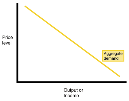
Aggregate Demand
- Shows the amount of Real GDP that the private, public, and foreign sector collectively desire to purchase at each possible price level.
- Relationship between the price level and level of GDPr is inverse
3 Reasons AD is downward sloping
- Real-Balances Effect
- Interest-Rate Effect
- Foreign Purchases Effect
Shifts in AD
- Change in C, Ig, G, or Xn
- Multiplier effect that produces a greater change than the original change in the 4 components
- Increase in AD, shift right
- Decrease in AD, shift left
Net Exports
- Exchange Rates (International value of U.S. dollar)
- Strong dollar = More imports and Less Exports = (AD shift left)
- Weak dollar = fewer imports and more exports = (AD shift right)
Relative Income
- Strong Foreign Economies = More Exports = AD shift right
- Weak Foreign Economies = Less Exports = AD shift left
Aggregate Supply
- The level of Real GDP that firms will produce at each price level

Long-Run v. Short-Run
- Long-Run
- Period of time where input prices are flexible and adjust to changes in the price-level
- In the long-run, the level of Real GDP is independent from price level
- Short-Run
- Period of time where input prices are sticky and do not adjust to changes in the price-level
- Real GDP is directly related to the price level
Long-Run Aggregate Supply (LRAS)
- marks the level of FE in the economy (same as the PPC)
- is always vertical at full employment
Changes in Short-Run Aggregate Supply (SRAS)
- increase in SRAS, shift to the right
- decrease, shift to the left
- the key to understanding shifts is per unit cost of production
- per-unit production cost = total input cost / total output
Determinants of SRAS
- Input prices = land, labor, machinery, ETC.
- Productivity = technology
Ranges of Aggregate Supply (AS)

Keynesian Range
- Horizontal
- Followers believe in a horizontal AS curve because when the economy is below FE, AD shifts out
- Increase in GDPr, UE drops, price level is constant
- Demand creates its own supply
Intermediate Range
- AS is between the Classical and Keynesian Range
- AS shifts outward, price level and GDPr increases
Classical Range
- Vertical
- In the long run, AS curve is vertical because the only effects of an increase in AD is when we are already at FE
- Increase in price level
- Supply creates its own demand (Say's Law)
Recessionary Gap - when equilibrium occurs below FE output

Inflationary Gap - when equilibrium occurs beyond FE output

Investment

- Money spent or expenditures on:
- New plants (factories)
- Capital equipment (machinery)
- Technology (hardware and software)
- New homes
- Inventories (goods sold by producers)
- Expected rates of return
- How does business make investment decisions?
- Cost/benefit analysis
- How does business determine the benefits?
- expected rate of return
- How does business count the cost?
- interest costs
- How does business determine the amount of investment they undertake?
- Compare expected rate of return to interest cost
- expected return > interest cost = invest
- expected return < interest cost = don't invest
- Real (r %) v. Nominal (i %)
- Nominal is the observable rate of interest
- Real subtracts out inflation and is only known ex post facto
- Compute r%
- = nominal - inflation
- Real interest rate (r%) determines the cost of investment decision
- Investment Demand Curve (ID)
- Downward sloping
- Why?
- when interest rate are high, fewer investments are profitable
- when ir are low, investments are profitable
- Shifts in ID
- Cost of production
- Business taxes
- Technology changes
- Stock of capital
- Expectations
- Consumption and Savings
- Disposable income (DI)
- income after taxes
- net imcome
- Consumption
- Household spending
- Ability to consume is constrained by: amount of DI and propensity to save
- DI = 0
- Dissaving
- Savings
- Household not spending
- Ability to save is constrained by: amount of DI and propensity to consume
- APS = average propensity to save
- APC = average propensity to consume
- APC + APS = 1
- APC > 1 dissaving
- MPC = marginal propensity to consume
- = change in consumption / change in DI
- MPS = marginal propensity to save
- = change in savings / change in DI
- MPS + MPC = 1
Determinants of C & S


- Wealth
- Expectations
- Household Debt
- Taxes
Spending Multiplier Effect
- an initial change in spending (C, Ig, G, Xn) causes a larger change in AD
- Multiplier - change in AD / change in spending
- 1 / MPS
- positive when increase in spending
- negative when decrease
Tax Multiplier
- when government taxes, the multiplier works in reverse
- money is leaving circular
- Multiplier (negative) = - MPC / MPS
Fiscal Policy
- Expansionary and Contractionary policy
- Deficits and surplus
- Built in stability
Changes in expenditures or tax revenues of the federal government
2 tools of fiscal policy
- Taxes - government can increase or decrease taxes
- Spending - government can increase/decrease spending
Fiscal policy is enacted to promote our nation's economic goods = FE, price stability, economic growth

Deficits, Surpluses, Debt
- Balanced Budget
- Revenues = Expenditures
- Budget deficit
- Revenues < expenditures
- Budget surplus
- Revenues > expenditures
- Government debt
- sum of all deficits - sum of all surpluses
- Government must borrow money when it runs into a deficit
- Borrows from individuals, corporations, financial institutions, foreign entities/governments
2 options of fiscal policy
- Discretionary Fiscal Policy (action)
- Expansionary (deficit)
- Contractionary (surplus)
- Non-discretionary (no action)
Discretionary v. Automatic FP
Discretionary
- increasing/decreasing government spending/taxes in order to return the economy to FE
- involves policymakers
Automatic
- UE compensation and marginal tax rates
- takes place without policymakers
Contractionary - policy designed to decrease AD
- strategy for controlling inflation
- decrease gov't spending/increase taxes
Expansionary - increase AD
- increasing GDP, combatting recession, reducing UE
- recession is countered with expansionary policy
- increase gov't spending/decrease taxes
Progressive Tax System
- Average tax rate (tax revenue/GDP) rises with GDP
Proportional Tax System
- Average tax rate remains constant as GDP changes
Regressive Tax System
- Average tax rate falls with GDP

The more progressive the tax system, the greater the economy's built-in stability